🍿 Quick Audio: Neo4j for IT Infrastructure

▶️ Video Guide

Note: This video and podcast was generated using AI, adapting the original content and technical insights created by the author of the Jax London blog post.

Although they aren’t entirely new and there are many established products on the market, graph databases have never really made it into the mainstream among developers. This is surprising, since negative experiences have rarely been reported. On the contrary: graph databases have been faithfully serving many production projects in the background for years. To understand the contexts where graph databases can fully show off their advantages, it’s worth looking at the theory behind the database.

Graph databases are suitable for storing highly interconnected datasets. The sample project accompanying this article provides a practical implementation of this kind of use case. It catalogs all IT systems used in an organization, along with the dependencies between them-such as those created by API calls. The graph also stores contact information for the systems so someone can be reached in the event of a system failure.

With this relatively simple dataset, a graph database can quickly and reliably answer very interesting questions:

• Which systems are indirectly affected by downtime in System X?
• Who can help me if the system at URL Y is unavailable?
• Which contact persons from calling systems must be available when an update is deployed to System Z?

This article explains the basics of graph databases using an example graph in Neo4j to address the requirements above. The second part of the series will demonstrate a concrete integration with Spring AI, a small UI, and the GraphRAG approach.

Basics

Graph databases are based on mathematical graph theory, whose origins date back to the 18th century. Graphs consist of just two elements: nodes and edges. In visual representations, circles represent the nodes and connecting lines represent the edges. Edges can be undirected or directed, visually represented by an arrow.

Graph database systems like Neo4j implement the concept of a labeled property graph: nodes carry one or more labels to clarify their role in the graph. Edges (referred to as relationships in this context) have a fixed type. Both elements carry any number of properties as key-value pairs.

Unlike pure graph theory, edges in Neo4j always have a direction. The example graph (Fig. 1) depicts the relevance of direction for the edge RUFT_AUF. In the example, the nodes are enriched with additional information. For instance, the systems carry a list of URLs where they can be reached. To facilitate identification, systems and people have a property where their name is stored.

First Steps

If you’re interested in a concrete hands-on experiment, you can get started right away. Simply save the lines from Listing 1 as _docker-compose.ym_l and run the command

_docker compose up_

to start an instance of Neo4j Community Edition. All scripts are also available in the sample project’s repository. The Neo4j Browser can be accessed in a web browser at the address localhost:7474. The login credentials stored in the Docker Compose file-the neo4j username and localpwd password-let you log in via the browser. For an environment that isn’t intended for only local access, you must assign a secure password.

Listing 1

_services:_

_neo4j-local:_

_image: neo4j:5-community_

_environment:_

_\- NEO4J_AUTH=neo4j/localpwd_

_ports:_

_\- "7474:7474"_

_\- "7687:7687"_

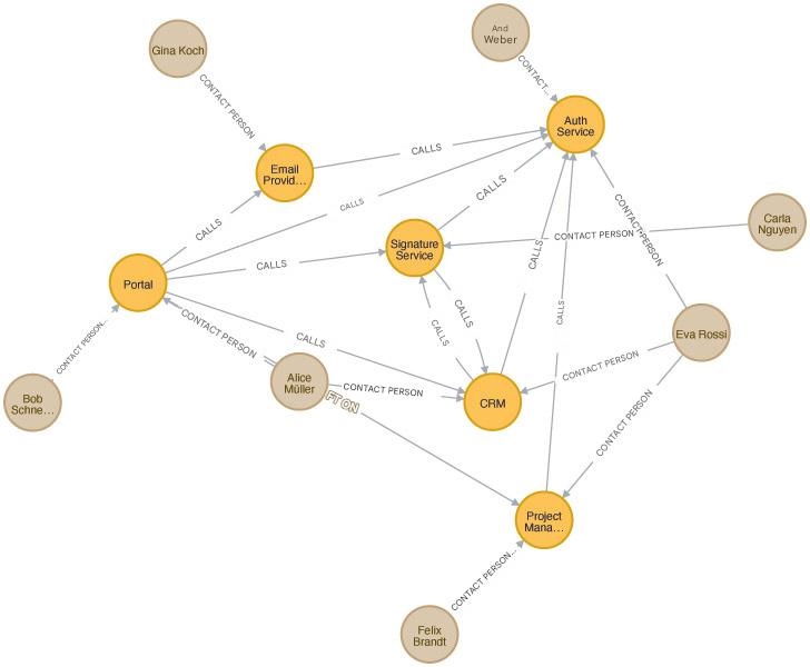
Fig. 1: Graph of the sample project

After logging in, the database is empty. The command in Listing 2 creates the initial graph for the sample project. After executing it in the browser, Neo4j displays the created graph; see Fig. 1. Neo4j’s interactive graph view lets users hide or show individual nodes and customize the graph’s display. The context menu lists the properties for the selected node or relationship (Fig. 2).

Listing 2

_CREATE_

_(portal:System {name: "Portal", external: false, urls: \["<https://portal.company.com"\]}>),_

_(auth:System {name: "Auth Service", external: false, urls: \["<https://auth.company.com"\]}>),_

_(signature:System {name: "Signature Service", external: false, urls: \["<https://sign.company.com"\]}>),_

_(crm:System {name: "CRM", external: true, urls: \["<https://crm.company.com"\]}>),_

_(tickets:System {name: "Project Management System", external: true, urls: \["<https://tickets.vendor.example/api>", "<https://tickets.company.com"\]}>),_

_(email:System {name: "Email Provider", external: true, urls: \["<https://email.vendor.example/v1/send"\]}>),_

_(alice:Person {name:"Alice Müller", email:"<[email protected]>"}),_

_(bob:Person {name:"Bob Schneider", email:"<[email protected]>"}),_

_(carla:Person {name:"Carla Nguyen", email:"<[email protected]>"}),_

_(dan:Person {name:"Dan Weber", email:"<[email protected]>"}),_

_(eva:Person {name:"Eva Rossi", email:"<[email protected]>"}),_

_(felix:Person {name:"Felix Brandt", email:"<[email protected]>"}),_

_(gina:Person {name:"Gina Koch", email:"<[email protected]>"}),_

_(portal)-\[:CALL\]->(signature),_

_(portal)-\[:CALL\]->(auth),_

_(portal)-\[:CALL\]->(tickets),_

_(portal)-\[:CALL\]->(email),_

_(portal)-\[:CALL\]->(crm),_

_(signature)-\[:CALL\]->(auth),_

_(signature)-\[:CALL\]->(crm),_

_(crm)-\[:CALL\]->(auth),_

_(crm)-\[:CALL\]->(signature),_

_(email)-\[:CALL\]->(auth),_

_(tickets)-\[:CALL\]->(auth),_

_(alice)-\[:CONTACT\]->(portal),_

_(alice)-\[:CONTACT\]->(crm),_

_(bob)-\[:CONTACT\]->(portal),_

_(carla)-\[:CONTACT\]->(signature),_

_(dan)-\[:CONTACT\]->(auth),_

_(eva)-\[:CONTACT\]->(auth),_

_(eva)-\[:CONTACT\]->(crm),_

_(eva)-\[:CONTACT\]->(tickets),_

_(felix)-\[:CONTACT\]->(tickets),_

_(gina)-\[:CONTACT\]->(email)_

_RETURN portal, auth, signature, crm, tickets, email, alice, bob, carla, dan, eva, felix, gina;_

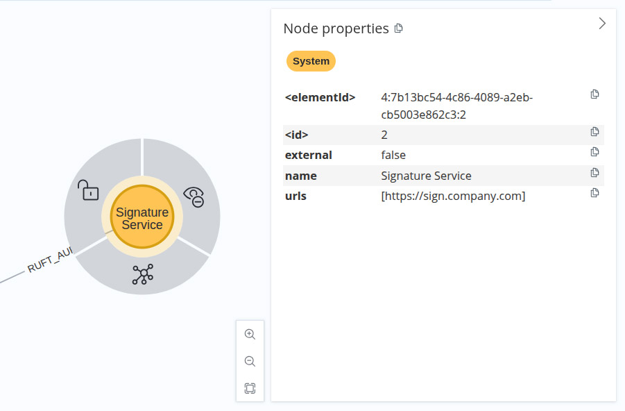
Fig. 2: Detailed view of a node

The CREATE statement does not include any constraints or indexes. In real-world projects, these constructs ensure that the dataset does not contain any duplicates. For larger datasets, manually selecting nodes with a UI is impractical, so a query language is needed.

Cypher: SQL for the graph

Relational databases have a justified and long history of success. As a query language, SQL has accompanied generations of computer scientists and supported countless analyses. In fact, relational databases respond quickly to a wide variety of queries through internal optimization, and we’ve learned to improve execution speed through indexing and schema optimization.

However, SQL reaches its limits when dealing with certain types of queries. While some SQL dialects provide recursive SQL constructs, these queries are not truly transparent or easy to manage.

In contrast, graph databases answer questions like: “Which systems are indirectly affected by System X’s downtime” with high efficiency. For many years, Neo4j has been developing Cypher, a query language optimized for property graphs. In 2024, the Graph Query Language (GQL) received the ISO standard ISO/IEC 39075:2024 as the query language for graph databases. Cypher’s ideas were significantly incorporated into the standards-and for good reason!

Cypher Basics

Cypher is especially impressive because of its intuitive syntax, which is based on the visual representation of a graph. Nodes are represented by parentheses: (s:System) selects all nodes labeled “System.” The parentheses create a visual link to the representation of nodes as circles in the graph. Consequently, an arrow represents the edges: -[:CONTACT]-> considers all relationships of the CONTACT type.

Cypher queries consist of these simple syntactic elements. Therefore, the query:

_MATCH (s:System) RETURN s.name, s.urls_

the names and URLs of all system nodes in the graph. This results in a table (Fig. 3).

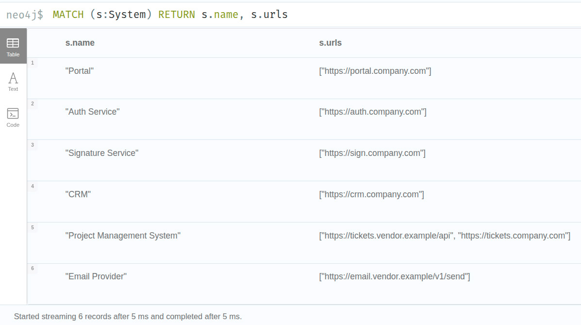
Fig. 3: Cypher query with tabular results

Admittedly, this example doesn’t have much advantage over SQL and a relational database. Things get more interesting when the query traverses a relationship path. The query’s syntax visually reflects the graph structure:

_MATCH (p:Person)-\[:CONTACT\]->(s:System) RETURN s, p_

The result, now a subgraph, no longer represents just individual nodes but their relationships as well. This is where the graph database truly shines. In this view, it’s immediately clear which individuals serve as contacts for multiple systems and which systems have redundant staff.

Searching and Filtering

In fact, the result of the previous query doesn’t differ from the whole graph (Fig. 1); the returned subgraph is the graph itself. But of course, Cypher can also filter for specific elements:

_MATCH (p:Person {name: "Alice Müller"})-\[:CONTACT\]->(s:System) RETURN p, s_;

This query returns the node for the person “Alice Müller” and all systems that she is the contact person for (Fig. 4). Cypher supports filtering by labels on both nodes and edges. This results in a true subgraph, which gives an easier-to-understand overview than a tabular representation.

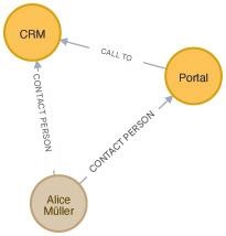
Fig. 4: Filtered graph

The query returns the same result.

_MATCH (p:Person)-\[:ANSPRECHPARTNER\]->(s:System)_

_WHERE p.name CONTAINS "Alice"_

_RETURN s, p;_

The WHERE syntax supports different kinds of comparison operations. The Cypher documentation gives a practical overview of the keywords and their usage.

Next-Level Cypher

These simple examples show Cypher’s accessibility. The visual similarity between the representation of nodes and edges makes it easier for beginners to get started. However, most of the examples can also be queried with a well-structured relational database.

Queries get really exciting when they delve to any depth into the relationship network. In the example graph, this includes querying which systems are directly or indirectly affected by downtime in a specific system.

_MATCH (x:System {name: "CRM"})<-\[:RUFT_AUF\*1..\]-(affected:System)_

_RETURN DISTINCT affected.name AS affectedSystem_

This query lists all systems that directly call the CRM, including all transitive callers. This is where the graph database really shines. This simple query identifies all dependencies even in complex datasets without needing explicit recursion. The tabular result lists all systems that would be affected by downtime in a given system.

In the modified version:

_MATCH (x:System {name: "CRM"})<-\[:RUFT_AUF\*1..\]-(affected:System)_

_RETURN x, affected_

Neo4j returns the result as a subgraph, which visualizes the call chains. Cypher notation supports the reading direction of the relationship.

Impact Analysis

Cypher also handles other practical questions with ease. The following query returns the points of contact for a specific system as a subgraph:

_MATCH (s:System {name: "CRM"})<-\[:CONTACT\]-(p:Person) RETURN s, p_

However, a far more pressing question is which contacts should be available when an update is installed on a specific system. For smooth operation, we should have at least one contact person available for every system directly or transitively dependent.

_MATCH (x:System {name: "CRM"})<-\[:CALL\*1..\]-(s:System)_

_OPTIONAL MATCH (p:Person)-\[:CONTACT\]->(s)_

_RETURN s.name AS affectedSystem, collect(DISTINCT p.name) AS contacts_

_ORDER BY affectedSystem;_

The OPTIONAL keyword ensures that systems with no CONTACT relation are also listed. In practice, this information is useful before an upcoming update.

More examples in the Movie Database

The Neo4j Docker image includes sample data and example queries. First, the guides (Fig. 5) create a graph in the database and introduce more complex query constructs with concrete examples. The :guide command in the query window opens the guide menu. The Movie Database is a good starting point to get an overview in just a few steps.

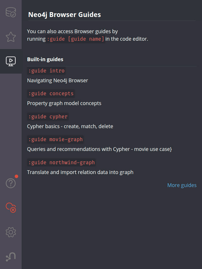
Fig. 5: Neo4j Guides

Solving Real-World Problems

After taking the first steps with a graph database, it’s surprising that this technology still remains a niche solution. Representing the data as a graph in the example graph is practically a given. Relationships play the central role in the data model. A list of systems can be quickly created in a tabular form. But the true value only becomes apparent through the explicit visualization of the relationships between systems and people.

Through various projects in past years, graph databases have proven that they can solve problems in a production-ready manner. One prominent example was their use in investigating the Panama Papers. But even in significantly smaller projects and with significantly smaller data sets, the technology demonstrates its strengths in practical application.

Key considerations for implementation

Graph databases should always be considered as option whenever the underlying data meets at least one of the following conditions:

• The informational value of the data lies primarily in the relationships between the data points.
• The data forms a network (e.g., delivery routes) or a tree-like/hierarchical structure.

Queries on data structured like this often require searches at varying levels of relationship depth. In the example graph, dependencies between systems may be direct, but they can also arise through several intermediate systems. A variable query can be efficiently executed using a graph database.

But if data usage focuses on aggregations, other database systems are better suited. It’s worth looking into alternatives for storing long, unstructured texts.

Interaction with business departments

Modeling relational databases always involves an intermediate step to translate business requirements into an abstract model-the schema. When addressing specific business questions, the information in the schema is translated back into the actual problem domain. This step is eliminated with graph databases. Engineers can discuss with business stakeholders at the whiteboard. The example graphs are directly incorporated into the software as test cases and can be transparently adapted by all participants if the framework conditions change.

The math behind the graph

Graph theory is rooted in mathematics. Over the decades, mathematicians have provided proofs and developed methods for searching within graphs. Graph database systems draw on these theoretical foundations and put them into practice. For example, Neo4j provides functions to determine the shortest path between two nodes. These mathematical insights make implementation reliable and high-performing.

Flexibility

Graph databases belong to the family of NoSQL databases. Like many others in this category, they are schema-optional. In principle, you can store data in any structure within the graph. New node labels and relationship types can be created quickly. This offers flexibility and speed during development. New, differently structured data is stored in the graph without needing to adapt a schema beforehand.

In its current versions, Neo4j supports constraints to enforce integrity rules in data management. Even the best data in a graph is useless if it cannot be retrieved. So, a pseudo-schema emerges through the definition of relationships and nodes in the specific project.

Graph Databases and AI

The unwavering hype for large language models (LLMs) is giving graph databases a new lease on life. In use cases beyond a simple chat, it’s common to provide the LLM with more context. Retrieval-augmented generation (RAG) is an established method with many effective implementation approaches.

Graph databases are increasingly emerging from their niche. Information stored in graphs provides excellent context for LLM queries. Context retrieval in particular is highly transparent and traceable. The second article in this series will focus on the GraphRAG method.

Conclusion

Graph databases are a serious alternative for data storage in modern software systems. When used thoughtfully and in the right context, they solve many problems that other database systems struggle with. Established solutions like Neo4j offer a gentle learning curve; visualization keeps abstraction to a minimum and provides quick successes. It makes working with graph databases truly enjoyable!

Outlook

The second part of this series integrates the example graph into a Spring project. Using Spring AI’s abstraction, we’ll create a small GraphRAG application that enriches text-based questions with information from the graph and answers them with an LLM. The result is an application that can answer who the contact person is for a system behind a given URL, even for users without Cypher knowledge. Until then, have fun taking your first steps in Neo4j!